Let’s be honest here. Can any of us say the last time we bought a car was fun? The satisfaction of driving away in your new vehicle was worth much more than the money you paid for it. As a result, I’m gonna try to cut out the middle man and give everyone a shot at a know-before-you-go opportunity. As long as you provide a few details on a car in question, I can return an accurate price that can save you plenty of time and resources.

When I bought the car I have right now, I wish I had some idea of the price range I’d be looking at given the specs of what I was wanting to buy. I searched through multiple dealerships and dealt with plenty of pushy salesmen. Once I landed in the lot of the car I purchased, I didn’t know I’d even be getting a car that day. I though it would be another dead end. They showed me a car that was not yet in the lot. They didn’t have a price for it yet and it took me about 5 hours before I was able to drive away. The car they presented me with was exactly what I wanted, but I had no idea what the cost was and I clearly paid the price (literally) just because I was tired of waiting. Mentally exhausted after that debacle, I felt driven to make sure that I could be more prepared than ever the next time I look for a new car.
I searched through droves of datasets looking for something that could help me with this task. I finally came across a dataset that was the perfect candidate. It displayed plenty of observations containing key features of a car. More importantly, it provided the MSRP for each and every vehicle in the dataset. All of this information transitioned me right to my question: how accurate can a Manufacturer Suggested Retail Price be predicted given a few specs of a desired car?
DRIVEN BY DATA
Exploring a dataset can be a tedious process, but I was determined to make this a useful and accurate model. I set a target variable quite easily knowing vehicle price was the only quanitity I wanted to predict. I explored the distribution of my data by these prices. To my surprise, this dataset contained prices ranging from $2,000 to $2,000,000; cars ranging from Toyota Camry’s to Bugatti Veyron’s. I knew right then that reduction of outliers in this data was a must. In a real world practical application, the price range for this data had to be confined, therefore, I reduced the data to cars priced less than $75,000. Many more data cleaning techniques later, I brought my dataset to a modest price range and adjusted other variables to allow for my models to make predictions with ease. I will continue to break down these techniques while explaining my workflow.
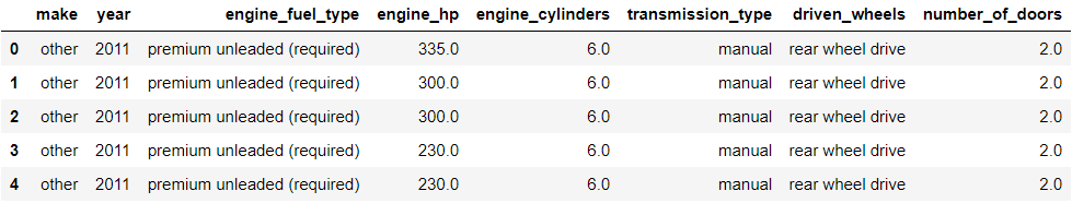
Above is just a small portion of what the data looked like after a fair amount of wrangling. I added some new columns that I though might help make more accurate predictions and, in turn, removed some columns that could allow for corruption, leaks, or unnecessary runtime in any of my chosen models. The final columns (not all are listed above) resulted in the perfect list of parameters that most people would already have defined for before going shopping.
RED LIGHT!
This workflow did not come without it’s complications however. During my attempt to create new variables that could help influence model prediction accuracy, I tried procuring a new column through some simple algebra for a new perspective. I received error after error. I had to iterate through each part of the process to figure out where the error was coming from. Through intense scrutiny, I discovered that this data contains cars with 0 cylinders. How? A portion of the data contained electric cars that only have an electric motor, therefore no cylinders. In the end, 0’s are not too friendly when it comes to algebra. I disregarded the new column and created a couple others instead.

MAKE AND MODEL?
Assuming there would only be one average price we could predict for any given car and it’s features (our baseline model), an average error of about $12,500 above or below the actual MSRP price took place in this data. Now I’m not confident about this, but I don’t think I’d be happy going to buy a car and find out that I’d possibly pay $12,000 more than what I thought. This is where the magic of machine learning models come into play. I deployed three different models in hopes that one would predict better than the rest, and that’s exactly what happened. On training and validation data (data we already know the answer to), a simple ridge regression model more than halved the baseline error, first by having an 80% validation accuracy, and predicted the MSRP within $5,500 above or below the true value. That seems reliable at first but, in comparison with a gradient boosting model that predicted within a range of $1,600 (and a 96% validation accuracy), simple does not seem like the right answer.

This more complex gradient boosting regression model had another boosting competitor (one with just under the same 96% validation accuracy score) but outperformed that one as well by $100 on prediction error. With this model, I began fine tuning it’s parameters to abstract the most accurate predictions possible. As a result, the model faced the test data and conquered predicting MSRP’s within a range of about $2,200 compared to the true value. That raises the question of how it performed worse on the test data when it did surprisingly well on the training data. There is really only one explanation: overfitting. This model, along with all of its training data, was trying very hard to predict every price with 100% accuracy that, when given new data it hasn’t seen before, the model had a hard time adjusting to make new predictions. However, there was still variance and error not being covered by the model (as explained in its 96% R-squared value), therefore we can, and should, actually rely on this model’s results.
AT THE FINISH LINE
In conclusion, however, the complications and time consuming wrangling techniques paid off. My final chosen model’s error averaged at $2,177 above or below the true MSRP value after being fitted to the testing data. Now, that is all fine and dandy but how did we get there? We can break down the steps and understand how the variables and values all interact within this model.
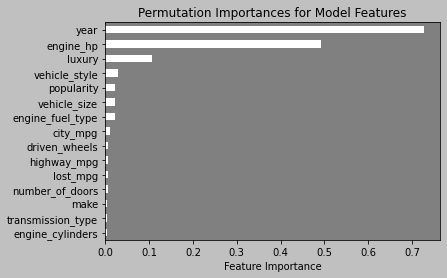
Above is a chart showing the importance of each column of this dataset on predicting a value with any given observation parameters. It is clear to see that the year of the car and it’s horsepower are two very important features. Due to the nature of the calculations, this graph displays that particular importance regardless of the model used on the data. No matter what methods we could use to predict a car’s price, these features will be just as important then as they are now. If we further decipher this ‘year’ column, we can begin to see how exactly the target values change in accordance with changes in year. To preface, a little bit of inference can be installed at this point by saying that, most likely, the newer the car is, the more expensive it will be. The graph below will tell us if we are right and will then put a face to the name.
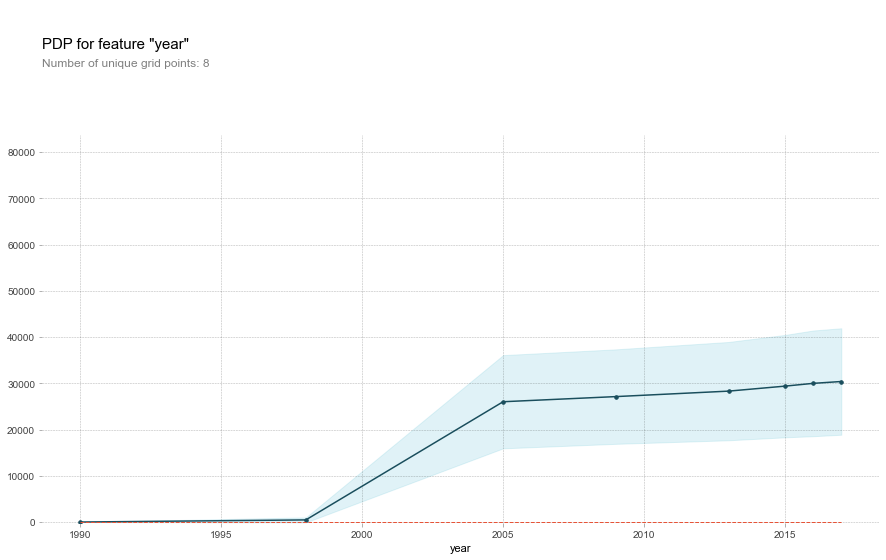
To no surprise, we see that price increases as year increases. Being able to look at the specifics, however, is the genius behind this graph. We see that the year really has no affect on predictions until around 1997 or 1998. Y2K seemed to have quite a stake in car sales considering it was the year that began boosting these costs. By the time 2005 rolls around, costs nearly level out increasing prices by about $30,000. Furthermore, when working in tandem with other features the ‘year’ variable continues to fascinate. Below we see how year affects the price when considering if a vehicle belongs (1) to the luxury market category or not (0).
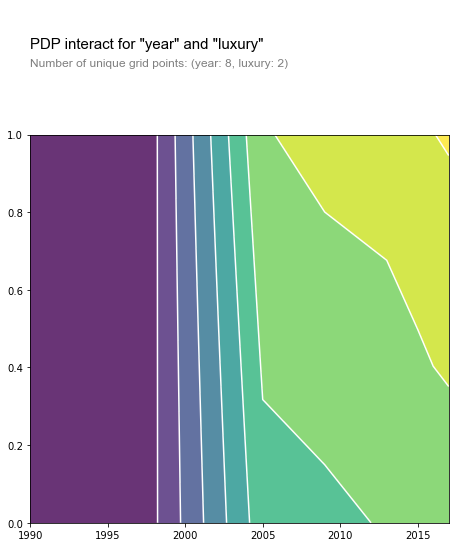
The yellow region in this heat map represents high MSRP’s while the purple represent cars that could be dirt cheap. Again to no surprise, cars in the luxury market category (values closest to 1 on the y-axis) cost more as year increases. What is interesting, however, is that cars considered ‘luxurious’ in years prior to around 2003-2005 (similar to the previous graph) still cost relatively nothing compared to those considered luxurious now.
At this point, imagine how much time we all could save by just exploring this data to fit our individual needs and take the results and run. There is an associated app with this article that will allow you to choose the exact parameters given in this data to your choosing so you can get the most information about your dream vehicle before any salesmen or shopping trips drain you of your time or energy. The link below provides all the details of the workflow and calculations through this process in the form of a Python notebook.
Check out the code notebook here.